Incompressible viscous hydrodynamics solver

pyro’s incompressible viscous solver solves:

\[\begin{split}\frac{\partial U}{\partial t} + U \cdot \nabla U + \nabla p &= \nu \nabla^2 U \\ \nabla \cdot U &= 0\end{split}\]

This solver is based on pyro’s incompressible solver, but modifies the velocity update step to take viscosity into account.

The main parameters that affect this solver are:

• section: [driver]

  option	value	description
  cfl	0.8

• section: [incompressible]

  option	value	description
  limiter	2	limiter (0 = none, 1 = 2nd order, 2 = 4th order)
  proj_type	2	what are we projecting? 1 includes -Gp term in U*

• section: [incompressible_viscous]

  option	value	description
  viscosity	0.1	kinematic viscosity of the fluid (units L^2/T)

• section: [particles]

  option	value	description
  do_particles	0
  particle_generator	grid

Examples

shear

The same shear problem as in incompressible solver, here with viscosity added.

pyro_sim.py incompressible_viscous shear inputs.shear

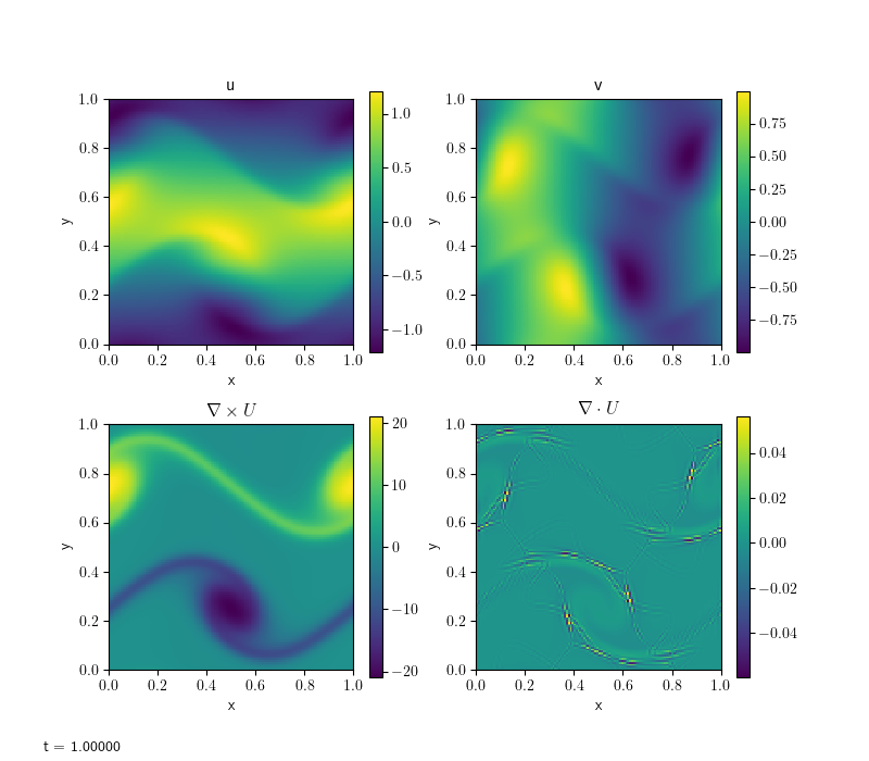
Compare this with the inviscid result. Notice how the velocities have diffused in all directions.

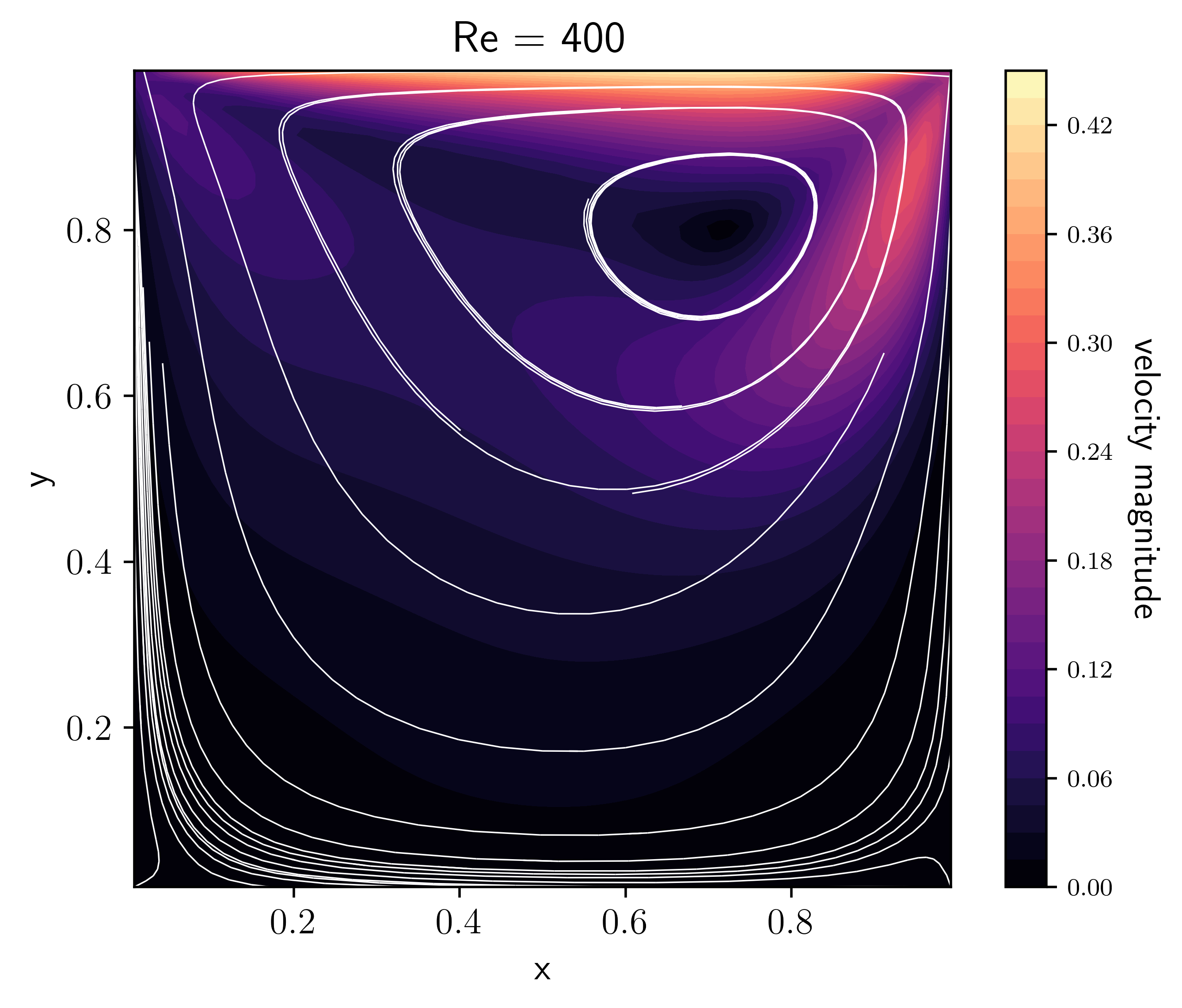
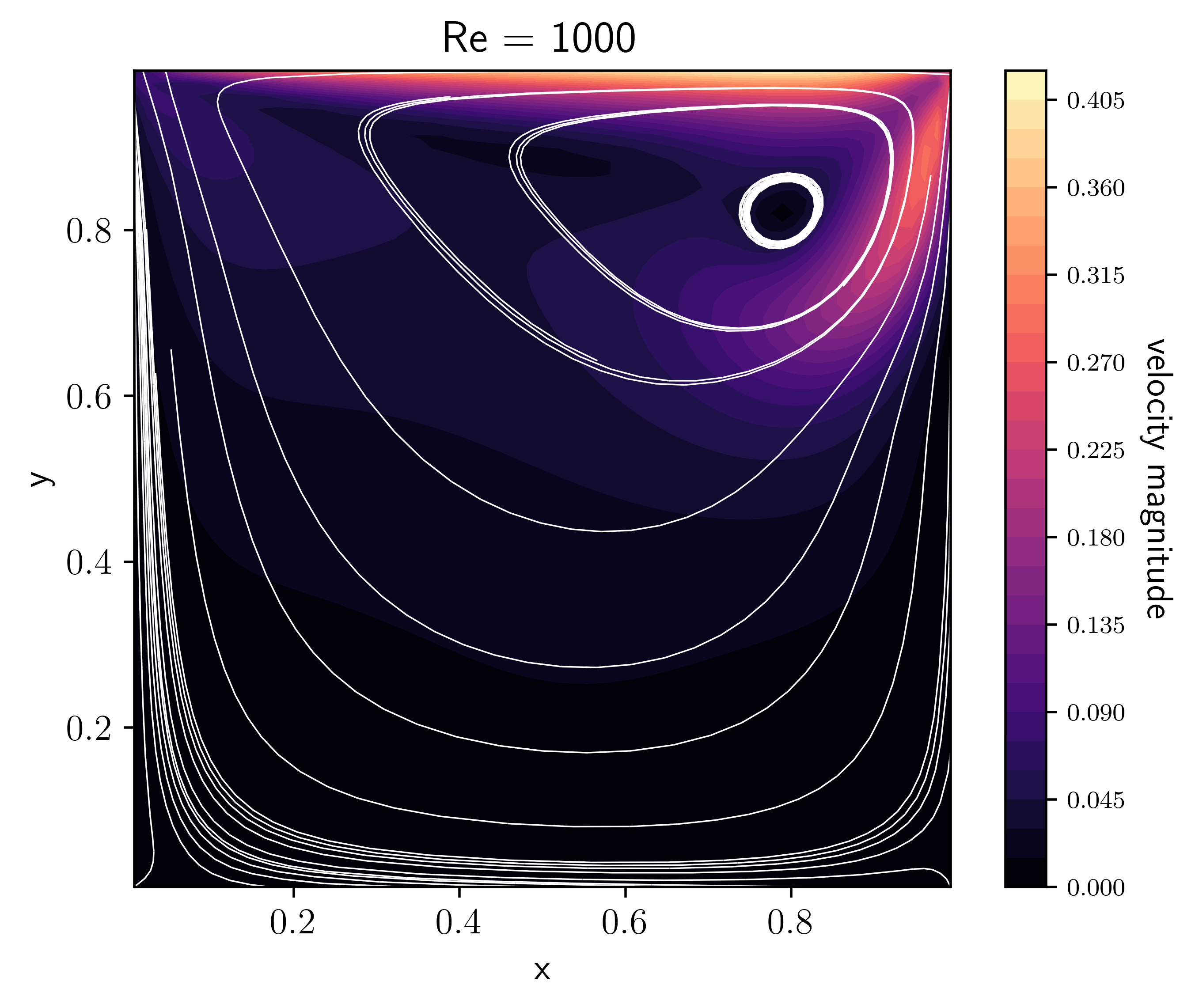
cavity

The lid-driven cavity is a well-known benchmark problem for hydro codes (see e.g. Ghia et al. [GhiaGhiaShin82], Kuhlmann and Romanò [KRomano19]). In a unit square box with initially static fluid, motion is initiated by a “lid” at the top boundary, moving to the right with unit velocity. The basic command is:

pyro_sim.py incompressible_viscous cavity inputs.cavity

It is interesting to observe what happens when varying the viscosity, or, equivalently the Reynolds number (in this case \(\rm{Re}=1/\nu\) since the characteristic length and velocity scales are 1 by default).

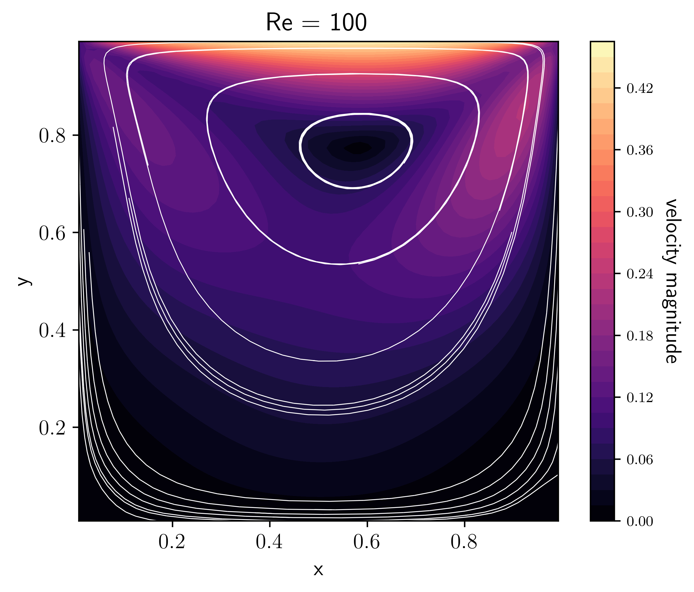
These plots were made by allowing the code to run for longer and approach a steady-state with the option driver.max_steps=1000, then running (e.g. for the Re=100 case):

python incompressible_viscous/problems/plot_cavity.py cavity_n64_Re100_0406.h5 -Re 100 -o cavity_Re100.png

convergence

This is the same test as in the incompressible solver. With viscosity, an exponential term is added to the solution. Limiting can again be disabled by adding incompressible.limiter=0 to the run command. The basic set of tests shown below are run as:

pyro_sim.py incompressible_viscous converge inputs.converge.32 vis.dovis=0
pyro_sim.py incompressible_viscous converge inputs.converge.64 vis.dovis=0
pyro_sim.py incompressible_viscous converge inputs.converge.128 vis.dovis=0

The error is measured by comparing with the analytic solution using the routine incomp_viscous_converge_error.py in analysis/. To generate the plot below, run

python incompressible_viscous/tests/convergence_errors.py convergence_errors.txt

or convergence_errors_no_limiter.txt after running with that option. Then:

python incompressible_viscous/tests/convergence_plot.py

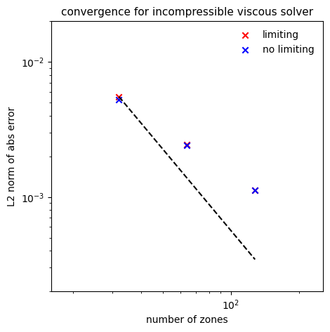
The solver is converging but below second-order, unlike the inviscid case. Limiting does not seem to make a difference here.

Exercises

Explorations

• In the lid-driven cavity problem, when does the solution reach a steady-state?

• [GhiaGhiaShin82] give benchmark velocities at different Reynolds number for the lid-driven cavity problem (see their Table I). Do we agree with their results?