Incompressible hydrodynamics

pyro has two different incompressible solvers: incompressible is inviscid and incompressible_viscous has viscosity.

incompressible solver

pyro’s incompressible solver solves:

\[\begin{split}\frac{\partial U}{\partial t} + U \cdot \nabla U + \nabla p &= 0 \\ \nabla \cdot U &= 0\end{split}\]

The algorithm combines the Godunov/advection features used in the advection and compressible solver together with multigrid to enforce the divergence constraint on the velocities.

Here we implement a cell-centered approximate projection method for solving the incompressible equations. At the moment, only periodic BCs are supported.

The main parameters that affect this solver are:

• section: [driver]

  option	value	description
  cfl	0.8

• section: [incompressible]

  option	value	description
  limiter	2	limiter (0 = none, 1 = 2nd order, 2 = 4th order)
  proj_type	2	what are we projecting? 1 includes -Gp term in U*

• section: [particles]

  option	value	description
  do_particles	0
  particle_generator	grid

supported problems

converge

Initialize a smooth incompressible convergence test. Here, the velocities are initialized as

\[ \begin{align}\begin{aligned}u(x,y) = 1 - 2 \cos(2 \pi x) \sin(2 \pi y)\\v(x,y) = 1 + 2 \sin(2 \pi x) \cos(2 \pi y)\end{aligned}\end{align} \]

and the exact solution at some later time t is then

\[ \begin{align}\begin{aligned}u(x,y,t) = 1 - 2 \cos(2 \pi (x - t)) \sin(2 \pi (y - t))\\v(x,y,t) = 1 + 2 \sin(2 \pi (x - t)) \cos(2 \pi (y - t))\\p(x,y,t) = -\cos(4 \pi (x - t)) - \cos(4 \pi (y - t))\end{aligned}\end{align} \]

The numerical solution can be compared to the exact solution to measure the convergence rate of the algorithm. These initial conditions come from Minion 1996.

shear

Initialize the doubly periodic shear layer (see, for example, Martin and Colella, 2000, JCP, 163, 271). This is run in a unit square domain, with periodic boundary conditions on all sides. Here, the initial velocity is:

\[\begin{split}u(x,y,t=0) = \begin{cases} \tanh(\rho_s (y - 1/4)) & \mbox{if}~ y \le 1/2 \\ \tanh(\rho_s (3/4 - y)) & \mbox{if}~ y > 1/2 \end{cases}\end{split}\]

\[v(x,y,t=0) = \delta_s \sin(2 \pi x)\]

parameters:

name	default
shear.rho_s	42.0
shear.delta_s	0.05

Examples

shear

The shear problem initializes a shear layer in a domain with doubly-periodic boundaries and looks at the development of two vortices as the shear layer rolls up. This problem was explored in a number of papers, for example, [BellColellaGlaz89] and [MartinColella00]. This is run as:

pyro_sim.py incompressible shear inputs.shear

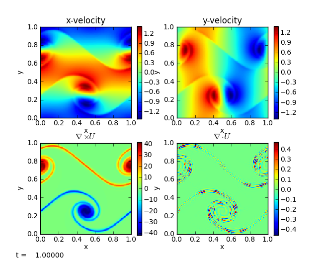
The vorticity panel (lower left) is what is usually shown in papers. Note that the velocity divergence is not zero—this is because we are using an approximate projection.

convergence

The convergence test initializes a simple velocity field on a periodic unit square with known analytic solution. By evolving at a variety of resolutions and comparing to the analytic solution, we can measure the convergence rate of the algorithm. The particular set of initial conditions is from [Minion96]. Limiting can be disabled by adding incompressible.limiter=0 to the run command. The basic set of tests shown below are run as:

pyro_sim.py incompressible converge inputs.converge.32 vis.dovis=0
pyro_sim.py incompressible converge inputs.converge.64 vis.dovis=0
pyro_sim.py incompressible converge inputs.converge.128 vis.dovis=0

The error is measured by comparing with the analytic solution using the routine incomp_converge_error.py in analysis/. To generate the plot below, run

python incompressible/tests/convergence_errors.py convergence_errors.txt

or convergence_errors_no_limiter.txt after running with that option. Then:

python incompressible/tests/convergence_plot.py

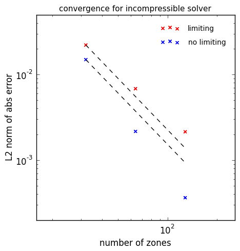
The dashed line is second order convergence. We see almost second order behavior with the limiters enabled and slightly better than second order with no limiting.

incompressible_viscous solver

pyro’s incompressible viscous solver solves:

\[\begin{split}\frac{\partial U}{\partial t} + U \cdot \nabla U + \nabla p &= \nu \nabla^2 U \\ \nabla \cdot U &= 0\end{split}\]

This is based on the incompressible solver, but modifies the velocity update step to take viscosity into account, by solving two parabolic equations (one for each velocity component) using multigrid.

The main parameters that affect this solver are:

• section: [driver]

  option	value	description
  cfl	0.8

• section: [incompressible]

  option	value	description
  limiter	2	limiter (0 = none, 1 = 2nd order, 2 = 4th order)
  proj_type	2	what are we projecting? 1 includes -Gp term in U*

• section: [incompressible_viscous]

  option	value	description
  viscosity	0.1	kinematic viscosity of the fluid (units L^2/T)

• section: [particles]

  option	value	description
  do_particles	0
  particle_generator	grid

supported problems

cavity

Initialize the lid-driven cavity problem. Run on a unit square with the top wall moving to the right with unit velocity, driving the flow. The other three walls are no-slip boundary conditions. The initial velocity of the fluid is zero.

Since the length and velocity scales are both 1, the Reynolds number is 1/viscosity.

References: https://doi.org/10.1007/978-3-319-91494-7_8 https://www.fluid.tuwien.ac.at/HendrikKuhlmann?action=AttachFile&do=get&target=LidDrivenCavity.pdf

converge

Initialize a smooth incompressible+viscous convergence test. Here, the velocities are initialized as

\[ \begin{align}\begin{aligned}u(x,y) = 1 - 2 \cos(2 \pi x) \sin(2 \pi y)\\v(x,y) = 1 + 2 \sin(2 \pi x) \cos(2 \pi y)\end{aligned}\end{align} \]

and the exact solution at some later time t, for some viscosity nu, is

\[ \begin{align}\begin{aligned}u(x,y,t) = 1 - 2 \cos(2 \pi (x - t)) \sin(2 \pi (y - t)) e^{-8 \pi^2 \nu t}\\v(x,y,t) = 1 + 2 \sin(2 \pi (x - t)) \cos(2 \pi (y - t)) e^{-8 \pi^2 \nu t}\\p(x,y,t) = - (\cos(4 \pi (x - t)) + \cos(4 \pi (y - t))) e^{-16 \pi^2 \nu t}\end{aligned}\end{align} \]

The numerical solution can be compared to the exact solution to measure the convergence rate of the algorithm.

shear

Initialize the doubly periodic shear layer (see, for example, Martin and Colella, 2000, JCP, 163, 271). This is run in a unit square domain, with periodic boundary conditions on all sides. Here, the initial velocity is:

\[\begin{split}u(x,y,t=0) = \begin{cases} \tanh(\rho_s (y - 1/4)) & \mbox{if}~ y \le 1/2 \\ \tanh(\rho_s (3/4 - y)) & \mbox{if}~ y > 1/2 \end{cases}\end{split}\]

\[v(x,y,t=0) = \delta_s \sin(2 \pi x)\]

parameters:

name	default
shear.rho_s	42.0
shear.delta_s	0.05

Examples

shear

The same shear problem as in incompressible solver, here with viscosity added.

pyro_sim.py incompressible_viscous shear inputs.shear

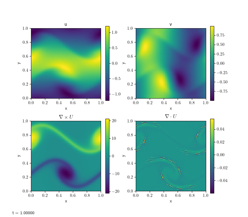
Compare this with the inviscid result. Notice how the velocities have diffused in all directions.

cavity

The lid-driven cavity is a well-known benchmark problem for hydro codes (see e.g. Ghia et al. [GhiaGhiaShin82], Kuhlmann and Romanò [KRomano19]). In a unit square box with initially static fluid, motion is initiated by a “lid” at the top boundary, moving to the right with unit velocity. The basic command is:

pyro_sim.py incompressible_viscous cavity inputs.cavity

It is interesting to observe what happens when varying the viscosity, or, equivalently the Reynolds number (in this case \(\rm{Re}=1/\nu\) since the characteristic length and velocity scales are 1 by default).

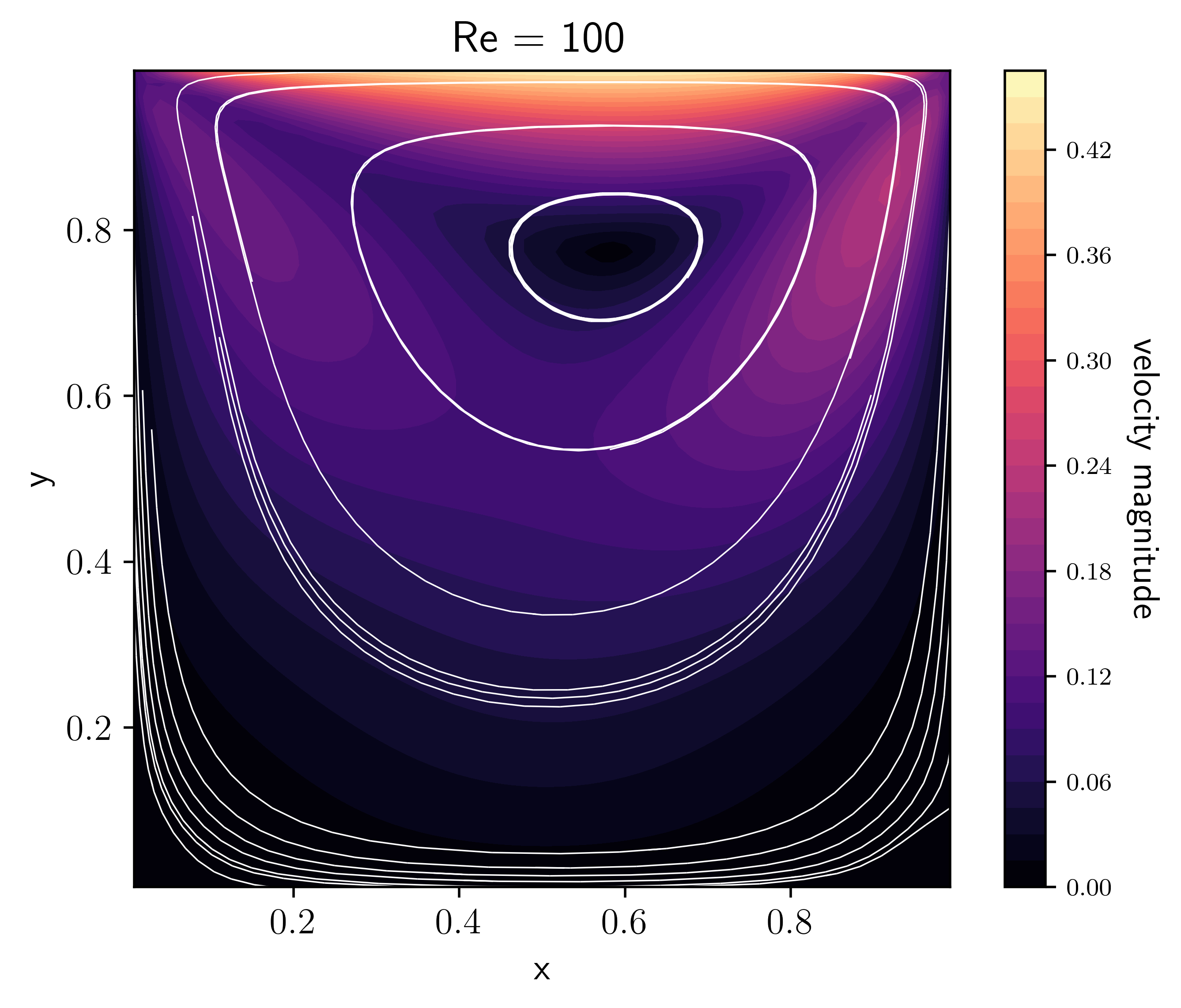
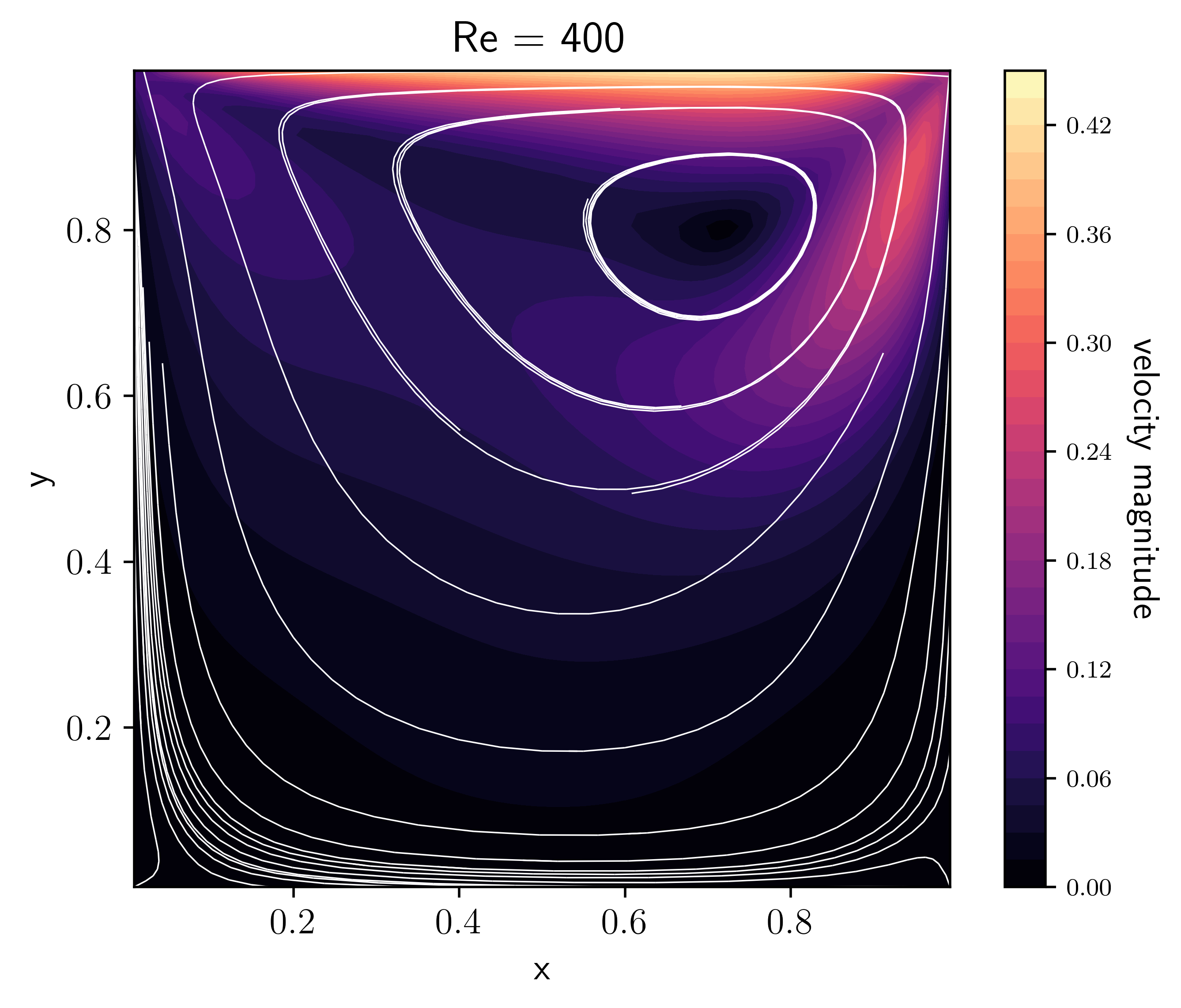
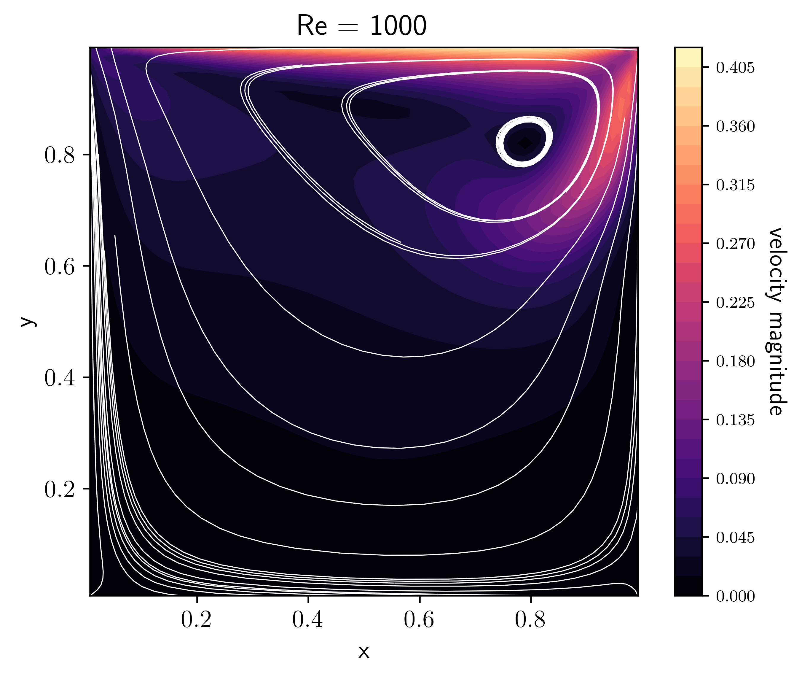
These plots were made by allowing the code to run for longer and approach a steady-state with the option driver.max_steps=1000, then running (e.g. for the Re=100 case):

python incompressible_viscous/problems/plot_cavity.py cavity_n64_Re100_0406.h5 -Re 100 -o cavity_Re100.png

convergence

This is the same test as in the incompressible solver. With viscosity, an exponential term is added to the solution. Limiting can again be disabled by adding incompressible.limiter=0 to the run command. The basic set of tests shown below are run as:

pyro_sim.py incompressible_viscous converge inputs.converge.32 vis.dovis=0
pyro_sim.py incompressible_viscous converge inputs.converge.64 vis.dovis=0
pyro_sim.py incompressible_viscous converge inputs.converge.128 vis.dovis=0

The error is measured by comparing with the analytic solution using the routine incomp_viscous_converge_error.py in analysis/. To generate the plot below, run

python incompressible_viscous/tests/convergence_errors.py convergence_errors.txt

or convergence_errors_no_limiter.txt after running with that option. Then:

python incompressible_viscous/tests/convergence_plot.py

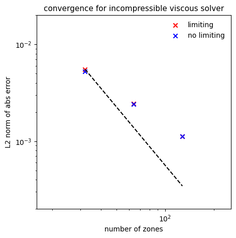
The solver is converging but below second-order, unlike the inviscid case. Limiting does not seem to make a difference here.

Exercises

Explorations

• Disable the MAC projection and run the converge problem—is the method still 2nd order?

• Disable all projections—does the solution still even try to preserve \(\nabla \cdot U = 0\)?

• Experiment with what is projected. Try projecting \(U_t\) to see if that makes a difference.

• In the lid-driven cavity problem, when does the solution reach a steady-state?

• [GhiaGhiaShin82] give benchmark velocities at different Reynolds number for the lid-driven cavity problem (see their Table I). Do we agree with their results?

Extensions

• Switch the final projection from a cell-centered approximate projection to a nodal projection. This will require writing a new multigrid solver that operates on nodal data.

• Switch to a variable density system. This will require adding a mass continuity equation that is advected and switching the projections to a variable-coefficient form (since ρ now enters).