Advection

The linear advection equation:

\[a_t + u a_x + v a_y = 0\]

provides a good basis for understanding the methods used for compressible hydrodynamics. Chapter 4 of the notes summarizes the numerical methods for advection that we implement in pyro.

pyro has several solvers for linear advection, which solve the equation with different spatial and temporal integration schemes.

advection solver

pyro.advection implements the directionally unsplit corner transport upwind algorithm [Colella90] with piecewise linear reconstruction. This is an overall second-order accurate method, with timesteps restricted by

\[\Delta t < \min \left \{ \frac{\Delta x}{|u|}, \frac{\Delta y}{|v|} \right \}\]

The parameters for this solver are:

• section: [advection]

  option	value	description
  u	1.0	advective velocity in x-direction
  v	1.0	advective velocity in y-direction
  limiter	2	limiter (0 = none, 1 = 2nd order, 2 = 4th order)

• section: [driver]

  option	value	description
  cfl	0.8	advective CFL number

• section: [particles]

  option	value	description
  do_particles	0
  particle_generator	grid

supported problems

smooth

Initialize a Gaussian profile (shifted so the minimum value is 1.0). This is smooth and the limiters should not kick in too much, so this can be used for testing convergence.

test

A problem setup for the unit testing.

tophat

Initialize a tophat profile—the value inside a small circular regions is set to 1.0 and is zero otherwise. This will exercise the limiters significantly.

advection_fv4 solver

pyro.advection_fv4 uses a fourth-order accurate finite-volume method with RK4 time integration, following the ideas in [McCorquodaleColella11]. It can be thought of as a method-of-lines integration, and as such has a slightly more restrictive timestep:

\[\Delta t \lesssim \left [ \frac{|u|}{\Delta x} + \frac{|v|}{\Delta y} \right ]^{-1}\]

The main complexity comes from needing to average the flux over the faces of the zones to achieve 4th order accuracy spatially.

The parameters for this solver are:

• section: [advection]

  option	value	description
  u	1.0	advective velocity in x-direction
  v	1.0	advective velocity in y-direction
  limiter	1	limiter (0 = none, 1 = ppm)
  temporal_method	RK4	integration method (see mesh/integrators.py)

• section: [driver]

  option	value	description
  cfl	0.8	advective CFL number

supported problems

advection_fv4 uses the problems defined by advection.

advection_nonuniform solver

pyro.advection_nonuniform models advection with a non-uniform velocity field. This is used to implement the slotted disk problem from [Zal79]. The basic method is similar to the algorithm used by the main advection solver.

The parameters for this solver are:

• section: [advection]

  option	value	description
  u	1.0	advective velocity in x-direction
  v	1.0	advective velocity in y-direction
  limiter	2	limiter (0 = none, 1 = 2nd order, 2 = 4th order)

• section: [driver]

  option	value	description
  cfl	0.8	advective CFL number

• section: [particles]

  option	value	description
  do_particles	0
  particle_generator	grid

supported problems

slotted

A circular profile with a rectangular slot cut out of it. This is meant to be run with the velocity field that causes it to rotate about the center, to understand how well we preserve symmetry.

parameters:

name	default
slotted.omega	0.5
slotted.offset	0.25

test

A test setup used for unit testing.

advection_rk solver

pyro.advection_rk uses a method of lines time-integration approach with piecewise linear spatial reconstruction for linear advection. This is overall second-order accurate, so it represents a simpler algorithm than the advection_fv4 method (in particular, we can treat cell-centers and cell-averages as the same, to second order).

The parameter for this solver are:

• section: [advection]

  option	value	description
  u	1.0	advective velocity in x-direction
  v	1.0	advective velocity in y-direction
  limiter	2	limiter (0 = none, 1 = 2nd order, 2 = 4th order)
  temporal_method	RK4	integration method (see mesh/integrators.py)

• section: [driver]

  option	value	description
  cfl	0.8	advective CFL number

supported problems

advection_rk uses the problems defined by advection.

advection_weno solver

pyro.advection_weno uses a WENO reconstruction and method of lines time-integration

The main parameters that affect this solver are:

• section: [advection]

  option	value	description
  u	1.0	advective velocity in x-direction
  v	1.0	advective velocity in y-direction
  limiter	0	Unused here, but needed to inherit from advection base class
  weno_order	3	k in WENO scheme
  temporal_method	RK4	integration method (see mesh/integrators.py)

• section: [driver]

  option	value	description
  cfl	0.5	advective CFL number

supported problems

advection_weno uses the problems defined by advection.

General ideas

The main use for the advection solver is to understand how Godunov techniques work for hyperbolic problems. These same ideas will be used in the compressible and incompressible solvers. This video shows graphically how the basic advection algorithm works, consisting of reconstruction, evolution, and averaging steps:

Examples

smooth

The smooth problem initializes a Gaussian profile and advects it with \(u = v = 1\) through periodic boundaries for a period. The result is that the final state should be identical to the initial state—any disagreement is our numerical error. This is run as:

pyro_sim.py advection smooth inputs.smooth

By varying the resolution and comparing to the analytic solution, we can measure the convergence rate of the method. The smooth_error.py script in analysis/ will compare an output file to the analytic solution for this problem.

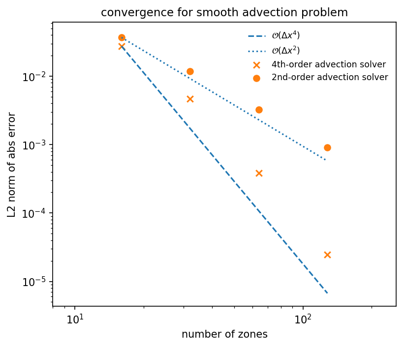
The points above are the L2-norm of the absolute error for the smooth advection problem after 1 period with CFL=0.8, for both the advection and advection_fv4 solvers. The dashed and dotted lines show ideal scaling. We see that we achieve nearly 2nd order convergence for the advection solver and 4th order convergence with the advection_fv4 solver. Departures from perfect scaling are likely due to the use of limiters.

Exercises

The best way to learn these methods is to play with them yourself. The exercises below are suggestions for explorations and features to add to the advection solver.

Explorations

• Test the convergence of the solver for a variety of initial conditions (tophat hat will differ from the smooth case because of limiting). Test with limiting on and off, and also test with the slopes set to 0 (this will reduce it down to a piecewise constant reconstruction method).

• Run without any limiting and look for oscillations and under and overshoots (does the advected quantity go negative in the tophat problem?)

Extensions

• Implement a dimensionally split version of the advection algorithm. How does the solution compare between the unsplit and split versions? Look at the amount of overshoot and undershoot, for example.

• Research the inviscid Burger’s equation—this looks like the advection equation, but now the quantity being advected is the velocity itself, so this is a non-linear equation. It is very straightforward to modify this solver to solve Burger’s equation (the main things that need to change are the Riemann solver and the fluxes, and the computation of the timestep).

  The neat thing about Burger’s equation is that it admits shocks and rarefactions, so some very interesting flow problems can be setup.