Defining our own problem in Jupyter

Here we explore how to add our own problem setup to a solver by writing the function to initialize the data outside of the pyro directory structure.

We’ll do the linear advection setup, but the idea is the same for any solver.

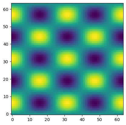
Let’s create the initial conditions:

\[\rho(x) = \cos(m \pi x / L) \sin(n \pi y / L)\]

where \(m\) is the number of wavelengths in \(x\) and \(n\) is in \(y\), and \(L\) is the domain width (which we’ll assume is 1).

We’ll call this problem setup “waves”

import numpy as np
import matplotlib.pyplot as plt

x = np.linspace(0, 1, 64)
y = np.linspace(0, 1, 64)

x2d, y2d = np.meshgrid(x, y, indexing="ij")

m = 4
n = 5
d = np.cos(m * np.pi * x2d) * np.sin(n * np.pi * y2d)

fig, ax = plt.subplots()
ax.imshow(d.T, origin="lower")

<matplotlib.image.AxesImage at 0x7fa394d916f0>

It often works best if you start with an existing problem. We can inspect the source of one of the build-in problems easily:

from pyro.advection.problems import smooth
smooth.init_data??

To define a problem, we need to create the init_data() function and a list of runtime parameters needed by the problem.

First the parameters–we’ll use \(m\) and \(n\) as the parameters we might want to set at runtime.

params = {"waves.m": 4, "waves.n": 5}

Our problem initialization routine gets a RuntimeParameters object passed in, so we can access these values when we do the initialization.

def init_data(my_data, rp):
    """ initialize the waves problem """

    dens = my_data.get_var("density")
    g = my_data.grid

    L_x = g.xmax - g.xmin
    L_y = g.ymax - g.ymin

    m = rp.get_param("waves.m")
    n = rp.get_param("waves.n")

    dens[:, :] = np.cos(m * np.pi * g.x2d / L_x) * \
                 np.sin(n * np.pi * g.y2d / L_y)

Now we can use our new problem setup. We need to register it with the solver by using the add_problem() method. Then everything works the same as any standard problem.

from pyro import Pyro

p = Pyro("advection")
p.add_problem("waves", init_data, problem_params=params)
p.initialize_problem("waves")

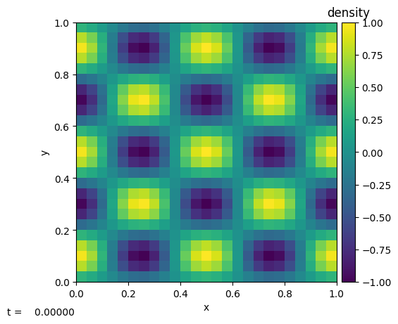
We can already look at the initial conditions

p.sim.dovis()

<Figure size 640x480 with 0 Axes>

If we wanted to change the number of wavelengths, we could override the default values of the runtime parameters when we call initialize_problem().

We also need to change the boundary conditions. For problems that we define this way, there is not a default “inputs” file that sets up the domain, etc. for us. But we can see what the default value of all the parameters for the simulation are:

print(p)

Solver = advection
Problem = waves
Simulation time = 0.0
Simulation step number = 0

Runtime Parameters
------------------
advection.limiter = 2
advection.u = 1.0
advection.v = 1.0
driver.cfl = 0.8
driver.fix_dt = -1.0
driver.init_tstep_factor = 0.01
driver.max_dt_change = 2.0
driver.max_steps = 10000
driver.tmax = 1.0
driver.verbose = 0
io.basename = pyro_
io.do_io = 0
io.dt_out = 0.1
io.force_final_output = 0
io.n_out = 10000
mesh.grid_type = Cartesian2d
mesh.nx = 25
mesh.ny = 25
mesh.xlboundary = reflect
mesh.xmax = 1.0
mesh.xmin = 0.0
mesh.xrboundary = reflect
mesh.ylboundary = reflect
mesh.ymax = 1.0
mesh.ymin = 0.0
mesh.yrboundary = reflect
particles.do_particles = 0
particles.n_particles = 100
particles.particle_generator = grid
vis.dovis = 0
vis.store_images = 0
waves.m = 4
waves.n = 5

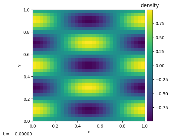
The main thing we need to change is the boundary conditions–we’ll make them periodic. We’ll also set the grid size to \(32^2\).

p = Pyro("advection")
p.add_problem("waves", init_data, problem_params=params)
p.initialize_problem("waves",
                     inputs_dict={"mesh.nx": 32,
                                  "mesh.ny": 32,
                                  "mesh.xlboundary": "periodic",
                                  "mesh.xrboundary": "periodic",
                                  "mesh.ylboundary": "periodic",
                                  "mesh.yrboundary": "periodic",
                                  "waves.m": 2})
p.sim.dovis()

<Figure size 640x480 with 0 Axes>

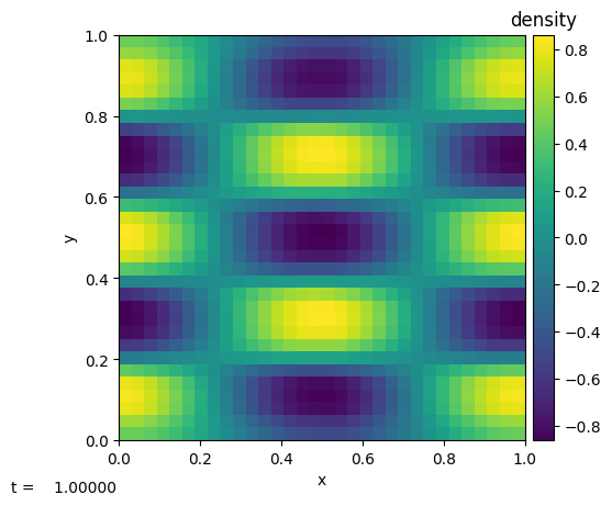
Now let’s evolve it

p.run_sim()
p.sim.dovis()

<Figure size 640x480 with 0 Axes>

The simulation is quite coarse, so the extrema are clipped a bit from the initial values, but we can fix that by increasing mesh.nx and mesh.ny.