Shallow water hydrodynamics#
The (augmented) shallow water equations take the form:
with \(h\) is the fluid height, \(U\) the fluid velocity, \(g\) the gravitational acceleration and \(\psi = \psi(x, t)\) represents some passive scalar.
swe solver#
The pyro swe implementation has flattening at shocks and a choice of Riemann solvers.
The main parameters that affect this solver are:
section:
[driver]option
value
description
cfl0.8section:
[particles]option
value
description
do_particles0particle_generatorgridsection:
[swe]option
value
description
use_flattening0apply flattening at shocks (1)
cvisc0.1artificial viscosity coefficient
limiter2limiter (0 = none, 1 = 2nd order, 2 = 4th order)
grav1.0gravitational acceleration (in y-direction)
riemannRoeHLLC or Roe
supported problems#
acoustic_pulse#
parameters:
name |
default |
|---|---|
|
1.4 |
|
0.14 |
advect#
dam#
parameters:
name |
default |
|---|---|
|
x |
|
1.0 |
|
0.125 |
|
0.0 |
|
0.0 |
kh#
parameters:
name |
default |
|---|---|
|
1.0 |
|
-1.0 |
|
2.0 |
|
1.0 |
logo#
quad#
parameters:
name |
default |
|---|---|
|
1.5 |
|
0.0 |
|
0.0 |
|
0.532258064516129 |
|
1.206045378311055 |
|
0.0 |
|
0.137992831541219 |
|
1.206045378311055 |
|
1.206045378311055 |
|
0.532258064516129 |
|
0.0 |
|
1.206045378311055 |
|
0.5 |
|
0.5 |
test#
Examples#
dam#
The dam break problem is a standard hydrodynamics problem, analogous to the Sod shock tube problem in compressible hydrodynamics. It considers a one-multidimensional problem of two regions of fluid at different heights, initially separated by a dam. The problem then models the evolution of the system when this dam is removed. As for the Sod problem, there exists an exact solution for the dam break problem, so we can check our solution against the exact solutions. See Toro’s shallow water equations book for details on this problem and the exact Riemann solver.
Because it is one-dimensional, we run it in narrow domains in the x- or y-directions. It can be run as:
pyro_sim.py swe dam inputs.dam.x
pyro_sim.py swe dam inputs.dam.y
A simple script, dam_compare.py in analysis/ will read a pyro
output file and plot the solution over the exact dam break solution
(as given by [SL58] and [WHZ99]). Below we see
the result for a dam break run with 128 points in the x-direction, and
run until t = 0.3 s.
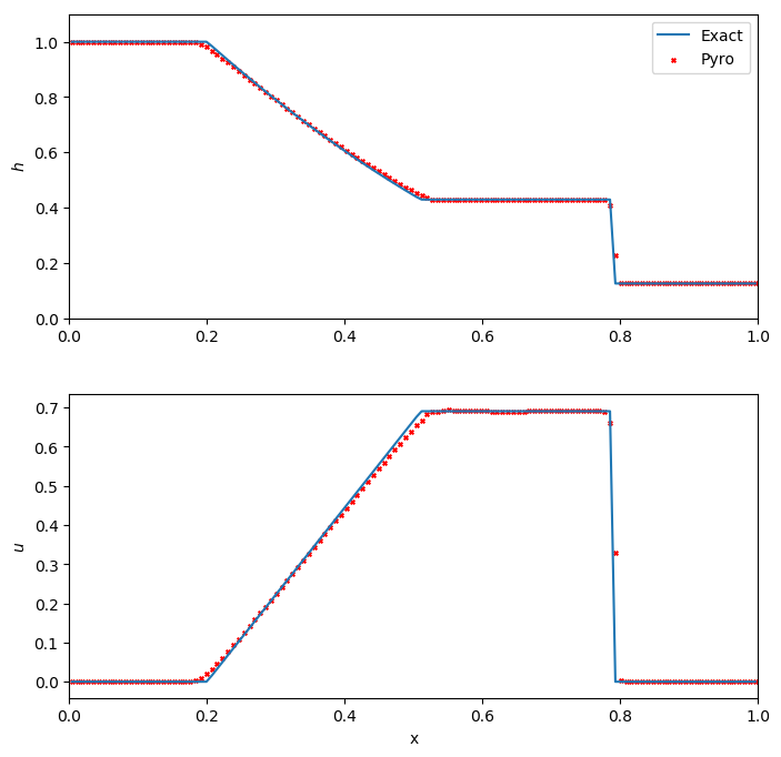
We see excellent agreement for all quantities. The shock wave is very steep, as expected. For this problem, the Roe-fix solver performs slightly better than the HLLC solver, with less smearing at the shock and head/tail of the rarefaction.
Exercises#
Explorations#
There are multiple Riemann solvers in the swe algorithm. Run the same problem with the different Riemann solvers and look at the differences. Toro’s shallow water text is a good book to help understand what is happening.
Run the problems with and without limiting—do you notice any overshoots?
Extensions#
Limit on the characteristic variables instead of the primitive variables. What changes do you see? (the notes show how to implement this change.)
Add a source term to model a non-flat sea floor (bathymetry).