Gravity and Hydrostatic Equilibrium

Here we explore the reconstruction of the pressure when in hydrostatic equilibrium.

Source terms in PPM

In the original PPM algorithm, the source terms (including gravity) were included in the characteristic projection. If we write our system as:

\[{\bf U}_t + [{\bf F}({\bf U})]_x = {\bf S}\]

The primitive variable equations would be:

\[{\bf q}_t + {\bf A}({\bf q}) {\bf q}_x = {\bf H}\]

where \({\bf H}\) are the sources for the primitive variables.

The interface states with sources included in the tracing appear as:

\[{\bf q}_{i+1/2,L}^{n+1/2} = \tilde{{\bf q}}_+ - \sum_{\nu;\lambda^{(\nu)}\ge 0} {\bf l}_i^{(\nu)} \cdot \left ( \tilde{{\bf q}}_+ - \mathcal{I}_+^{(\nu)}({\bf q}_i) - \frac{\Delta t}{2} \mathcal{I}_+^{(\nu)}({\bf H}_i) \right ) {\bf r}_i^{(\nu)}\]

\[{\bf q}_{i-1/2,R}^{n+1/2} = \tilde{{\bf q}}_- - \sum_{\nu;\lambda^{(\nu)}\le 0} {\bf l}_i^{(\nu)} \cdot \left ( \tilde{{\bf q}}_+ - \mathcal{I}_-^{(\nu)}({\bf q}_i) - \frac{\Delta t}{2} \mathcal{I}_-^{(\nu)}({\bf H}_i) \right ) {\bf r}_i^{(\nu)}\]

For gravity, \({\bf H}\) is only non-zero for velocity, so only the velocity interface states will see this contribution.

Note

We use a factor of 1/2 in front of the source term to time-center it–this is in contrast to the original PPM paper, and seems necessary to get 2nd order

The hse problem setup

Here we’ll look at the hse problem setup. This initializes a 1D isothermal atmosphere in hydrostatic equilibrium with constant gravity. If we start out with zero-velocity, then there should be no accelerations and the velocity should remain zero and the atmosphere static. This allows us to test how well our methods preserve HSE.

from ppmpy.euler import Euler
from ppmpy.gravity import constant_gravity
from ppmpy.initial_conditions import hse

import matplotlib.pyplot as plt
import numpy as np

Here are the parameters needed for the atmosphere initialization:

params = {"base_density": 1.0, "base_pressure": 1.0, "g_const": -1.0}

Let’s look at the initial atmosphere

nx = 64
e = Euler(nx, 0.5, init_cond=hse,
          grav_func=constant_gravity,
          bc_left_type="reflect", bc_right_type="reflect", params=params)
fig = e.plot_prim()

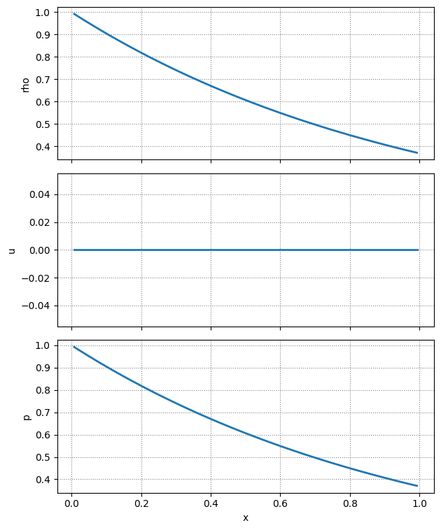
Notice that we are using reflecting boundaries at the top and bottom of the atmosphere.

Important

We want the reconstruction to guarantee that there is no flux through the boundaries when doing reflection. This means that we need to do odd-reflection on gravity (just like with velocity) to ensure that the source term tracing at the lower boundary is balanced.

We also explicitly enforce reflection on the interface states. On the left:

\[\begin{align*} {\rho}_{{\tt lo}-1/2,L} &= {\rho}_{{\tt lo}-1/2,R} \\ {u}_{{\tt lo}-1/2,L} &= -{u}_{{\tt lo}-1/2,R} \\ {p}_{{\tt lo}-1/2,L} &= {p}_{{\tt lo}-1/2,R} \end{align*}\]

and on the right:

\[\begin{align*} {\rho}_{{\tt hi}+1/2,R} &= {\rho}_{{\tt hi}+1/2,L} \\ {u}_{{\tt hi}+1/2,R} &= -{u}_{{\tt hi}+1/2,L} \\ {p}_{{\tt hi}+1/2,R} &= {p}_{{\tt hi}+1/2,L} \end{align*}\]

Normal PPM reconstruction

Here we use reflecting boundaries and the standard PPM reconstruction, with limiting.

nx = 16
e = Euler(nx, 0.5, init_cond=hse,
          grav_func=constant_gravity,
          bc_left_type="reflect", bc_right_type="reflect", params=params)

We can look at the reflecting boundary conditions to see what they do to the atmosphere

fig, ax = plt.subplots()
q = e.cons_to_prim()
ax.plot(e.grid.x, q[:, e.v.qp], marker="x")
ax.set_ylabel("p")
ax.set_xlabel("x")

Text(0.5, 0, 'x')

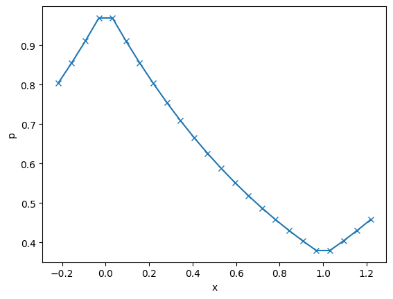
Now we can visualize how PPM reconstructs pressure near the lower boundary

gp = e.grid.draw(lo_index=3, hi_index=8, stretch=2)
e.draw_prim(gp, e.v.qp)

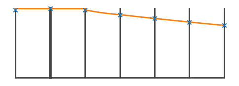
Notice that the first interior zone has a flat profile, so there is no pressure gradient and that zone will not be in HSE when we use the pressure coming from the Riemann problem to balance the gravitational source term.

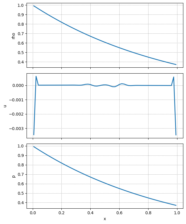
Let’s evolve this for 0.5 s to see how well HSE is maintained

nx = 64
e = Euler(nx, 0.5, init_cond=hse,
          grav_func=constant_gravity,
          bc_left_type="reflect", bc_right_type="reflect", params=params)
e.evolve(0.5, verbose=False)
fig = e.plot_prim()

Hydrostatic pressure reconstruction

Now we explore the case where we have the PPM reconstruction understand HSE. If we consider the initial cubic interpolation to find \({\bf q}_{i\pm 1/2}\) for zone \(i\), we can write that as:

\[{\bf q}_{i+1/2} = f({\bf q}_{i-1}, {\bf q}_{i}, {\bf q}_{i+1}, {\bf q}_{i+2})\]

\[{\bf q}_{i-1/2} = f({\bf q}_{i-2}, {\bf q}_{i-1}, {\bf q}_{i}, {\bf q}_{i+1})\]

For the pressure, we modify the \({\bf p}\) seen by the cubic by subtracting off HSE integrating from zone \(i\):

\[p^\prime_i = 0\]

\[p^\prime_{i\pm 1} = p_{i\pm 1} - \int_{x_i}^{x_{i\pm 1}} \rho g dx\]

\[p^\prime_{i\pm 2} = p_{i\pm 2} - \int_{x_i}^{x_{i\pm 2}} \rho g dx\]

where we treat \(\rho\) and \(g\) as piecewise constant within a zone when doing the integral.

We then do the cubic interpolation on \(p^\prime\). We can then either add back the HSE pressure or leave it as a perturbation.

First we’ll consider the case where we add back the HSE pressure. We use these values of \(p^\prime_{i\pm 1/2}\) to define the parabola edges:

\[p^\prime_- = p^\prime_{i-1/2}\]

\[p^\prime_+ = p^\prime_{i+1/2}\]

and then do the PPM limiting on them as needed. We then add back the HSE pressure to the parabola edge values:

\[p_- = p^\prime_- + p_i - \frac{\Delta x}{2} \rho_i g_i\]

\[p_+ = p^\prime_+ + p_i + \frac{\Delta x}{2} \rho_i g_i\]

Note

With this HSE reconstruction, the interface state \({\bf q}_{i+1/2}\) seen by zone \(i\) immediately after the cubic interpolation is no longer the same as that seen by zone \(i+1\).

Tip

This reconstruction is done by the HSEPPMInterpolant class, and used within Euler when use_hse_construction=True is set.

nx = 16
e = Euler(nx, 0.5, init_cond=hse,
          grav_func=constant_gravity,
          use_hse_reconstruction=True,
          bc_left_type="reflect", bc_right_type="reflect", params=params)

gp2 = e.grid.draw(lo_index=3, hi_index=8, stretch=2)
e.draw_prim(gp2, e.v.qp)

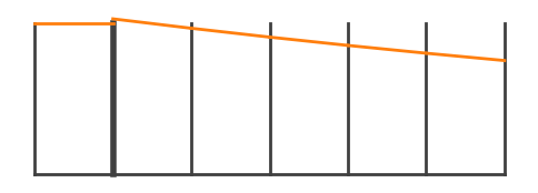
In this case, we see that the pressure in the first interior zone has a gradient that matches the needed HSE pressure gradient.

Now let’s evolve this to see how well HSE is maintained with this reconstruction

nx = 64
e = Euler(nx, 0.5, init_cond=hse,
          grav_func=constant_gravity,
          use_hse_reconstruction=True,
          bc_left_type="reflect", bc_right_type="reflect", params=params)
e.evolve(0.5, verbose=False)
fig = e.plot_prim()

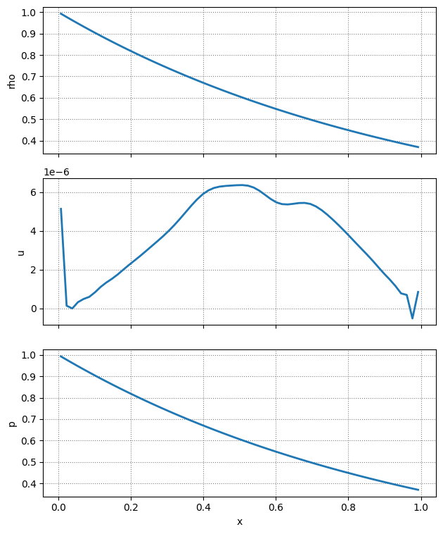
It is much better–the velocity is 3 orders-of-magnitude smaller. But we can actually do better if we don’t include the HSE pressure in the characteristic projection.

Addressing characteristic tracing

The final variation is to keep the parabola in terms of \(p^\prime\) and do the characterstic tracing on that. Then we need add back in the HSE interface pressure after the tracing.

A few notes:

• We need to add back in the HSE pressure when computing the eigenvectors from the reference state.

• We do not include the gravitational source term in the characteristic tracing, since it is taken into account by tracing \(p^\prime\).

• After adding up all of the jumps carried by the 3 waves, we need to add the HSE interface pressure back to the interfaces.

This results in a well-balanced method.

Note

This method is enabled by setting hse_as_perturbation=True together with use_hse_reconstruction=True

nx = 64
e = Euler(nx, 0.5, init_cond=hse,
          grav_func=constant_gravity,
          use_hse_reconstruction=True, hse_as_perturbation=True,
          bc_left_type="reflect", bc_right_type="reflect", params=params)
e.evolve(0.5, verbose=False)
fig = e.plot_prim()

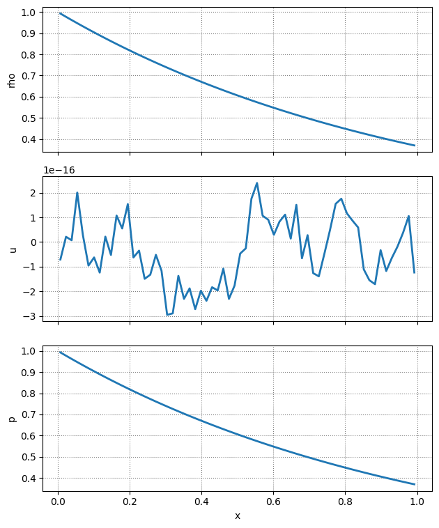
Now we see that the velocity is zero to machine precision.