Particles

A solver for modelling particles.

particles.particles implementation and use

We import the basic particles module functionality as:

import particles.particles as particles

The particles solver is made up of two classes:

• Particle, which holds the data about a single particle (its position and velocity);

• Particles, which holds the data about a collection of particles.

The particles are stored as a dictionary, and their positions are updated based on the velocity on the grid. The keys are tuples of the particles’ initial positions (however the values of the keys themselves are never used in the module, so this could be altered using e.g. a custom particle_generator function without otherwise affecting the behaviour of the module).

The particles can be initialized in a number of ways:

• randomly_generate_particles, which randomly generates n_particles within the domain.

• grid_generate_particles, which will generate approximately n_particles equally spaced in the x-direction and y-direction (note that it uses the same number of particles in each direction, so the spacing will be different in each direction if the domain is not square). The number of particles will be increased/decreased in order to fill the whole domain.

• array_generate_particles, which generates particles based on array of particle positions passed to the constructor.

• The user can define their own particle_generator function and pass this into the Particles constructor. This function takes the number of particles to be generated and returns a dictionary of Particle objects.

We can turn on/off the particles solver using the following runtime parameters:

[particles]
do_particles	do we want to model particles? (0=no, 1=yes)
n_particles	number of particles to be modelled
particle_generator	how do we initialize the particles? “random” randomly generates particles throughout the domain, “grid” generates equally spaced particles, “array” generates particles at positions given in an array passed to the constructor. This option can be overridden by passing a custom generator function to the Particles constructor.

Using these runtime parameters, we can initialize particles in a problem using the following code in the solver’s Simulation.initialize function:

if self.rp.get_param("particles.do_particles") == 1:
      n_particles = self.rp.get_param("particles.n_particles")
      particle_generator = self.rp.get_param("particles.particle_generator")
      self.particles = particles.Particles(self.cc_data, bc, n_particles, particle_generator)

The particles can then be advanced by inserting the following code after the update of the other variables in the solver’s Simulation.evolve function:

if self.particles is not None:
     self.particles.update_particles(self.dt)

This will both update the positions of the particles and enforce the boundary conditions.

For some problems (e.g. advection), the x- and y- velocities must also be passed in as arguments to this function as they cannot be accessed using the standard get_var("velocity") command. In this case, we would instead use

if self.particles is not None:
     self.particles.update_particles(self.dt, u, v)

Plotting particles

Given the Particles object particles, we can plot the particles by getting their positions using

particle_positions = particles.get_positions()

In order to track the movement of particles over time, it’s useful to ‘dye’ the particles based on their initial positions. Assuming that the keys of the particles dictionary were set as the particles’ initial positions, this can be done by calling

colors = particles.get_init_positions()

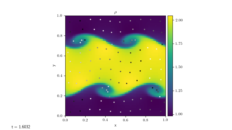
For example, if we color the particles from white to black based on their initial x-position, we can plot them on the figure axis ax using the following code:

particle_positions = particles.get_positions()

# dye particles based on initial x-position
colors = particles.get_init_positions()[:, 0]

# plot particles
ax.scatter(particle_positions[:, 0],
    particle_positions[:, 1], s=5, c=colors, alpha=0.8, cmap="Greys")

ax.set_xlim([myg.xmin, myg.xmax])
ax.set_ylim([myg.ymin, myg.ymax])

Applying this to the Kelvin-Helmholtz problem with the compressible solver, we can produce a plot such as the one below, where the particles have been plotted on top of the fluid density.